The what? It’s the formula for inverting the Mercator projection in the latitude direction. I’ve recently added to LogMyGsm a display of the latitude at the point in the centre of the map display. The internal coordinates are in Web Mercator space to ease the map tile handling. To get the latitude for display, the gd(Y) operation has to be applied.
The standard formula to return degrees latitude from the Y coordinate of the projection is gd(Y), coded thus:
static inline double exact_lat(double y)
{
    double t = (1.0 - 2.0*y)*M_PI;
    double M = (2.0* atan(exp(t))) - 0.5*M_PI;
    return M*(180.0/M_PI);
}
Given that this has to be run for every update as the map is dragged (so tens of updates a second possibly), the atan and exp might be a little wasteful. And optimising is fun…
The following is an approximation
#define P1 179.9989063857
#define P3 507.2276380744
#define P5 176.2675623673
#define Q0 1.0000000000
#define Q2 4.4623636863
#define Q4 4.2727924855
#define Q6 0.4175728442

static inline double approx_lat(double y)
{
    double z = 1.0 - 2.0*y;
    double z2 = z*z;
    double z4 = z2*z2;
    double t, b0, b4, b, t2;
    b4 = Q4 + Q6*z2;
    b0 = Q0 + Q2*z2;
    t2 = P3 + P5*z2;
    b = b0 + b4*z4;
    t = P1 + t2*z2;
    return z*t/b;
}
This looks like more code. However, there are no calls to the transcendental libm functions exp and atan here. On an x86-64 machine, this is more than 10x faster than the exact version. I’m hoping the conclusion would be similar on the Cortex-A9 and ARM11 in my 2 smartphones. To be confirmed!
As for the accuracy: it’s within 5e-5 degrees to beyond 71 degrees N/S, and within 7e-4 degrees between 71 and 85 degrees. So the accuracy up to 71 degrees is enough to give +/-1 in the 4th decimal place. There isn’t much habitable landmass beyond 71 degrees, so the accuracy there was compromised to improve the accuracy below 71 degrees.
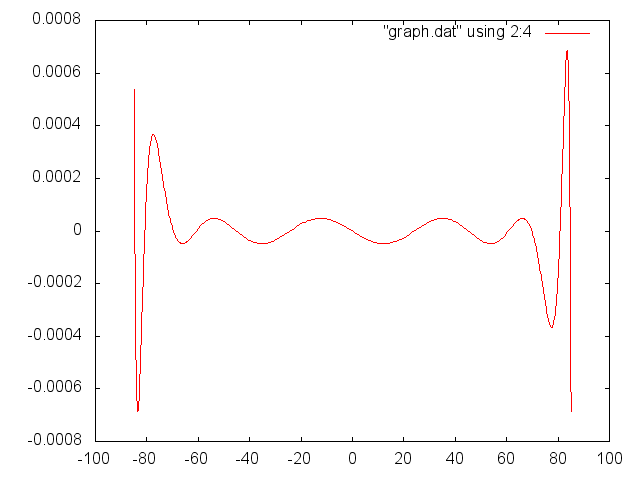
The degrees error versus latitude is shown in the above. Notice the nice equiripple error behaviour up to 71 degrees.
At some point I will need to write up the derivation properly. In outline : a pade approximation was computed by solving a set of linear equations at a set of Y values in [0,1]. The initial set of Y values were Chebyshev nodes. After each iteration, the Y values were adjusted to focus attention around the place with the greatest remaining error, and the procedure repeated. Luckily, this converged to the minimax solution shown.
